From 11:00 PM CST Friday, Apr 11th - 1:30 PM CST Saturday, Apr 12th, ni.com will undergo system upgrades that may result in temporary service interruption.
We appreciate your patience as we improve our online experience.
From 11:00 PM CST Friday, Apr 11th - 1:30 PM CST Saturday, Apr 12th, ni.com will undergo system upgrades that may result in temporary service interruption.
We appreciate your patience as we improve our online experience.
To download NI software, including the products shown below, visit ni.com/downloads.
This example presents a method used to recreate a signal from a set of Random sample points. It utilizes a compressive sampling algorithm to construct the signals most important portions. This example documents steps in the experimental process to prove the algorithm being presented.
This Compressive Data Acquisition LabVIEW program presents a signal reconstruction algorithm from a set of single random (scalar) measurements, where the signal is k sparse in some transform domain. Each measurement or observation represents a random projection of the signal onto a single scalar value. By applying Discrete Radon Transform techniques, the original signal can be reconstructed from these random sampled measurements. However, this requires a very large set of measurements which defeats the purpose of compressive data acquisition. To acquire the wideband data below the Nyquist frequency, a rank order filter is applied in the sparse transform domain to extract the k most significant components.
Consider the basic compressive sampling relationship
 | (1) |
| where | y is an M-element vector R is an MxN random binary sampling matrix x is an N-element sampled vector x is k-sparse in some transform domain T 0 < k << N |
The elements of y are given by
 | (2) |
where ri,j is the jth element the ith R random binary sampling basis with probabilities
 | (3) |
 | (4) |
Equations (1) and (2) reveal a standard projection onto a single scalar measurement. Therefore x can be reconstructed from the y projections using
 | (5) |
To verify that equation (5) does indeed converge, a simulation was implemented in LabVIEW using
 | (6) |
and letting the systems run in an "infinite" loop. The original signal consisted of the sum of sinusoids. The frequency (sparse) domain results for 7 active components is shown in Fig. 1.
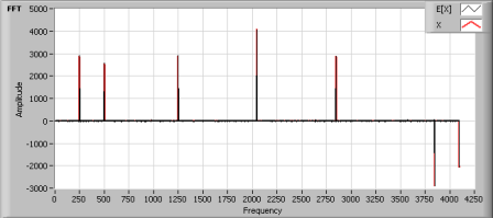
Fig. 1. Signal Convergence in the Sparse Domain
Clearly, we desire to reconstruct x from y from i samples such that i << N. To accelerate the convergence, a k-rank-order filter is applied in the signal's sparse domain. That is
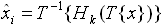 | (7) |
| where | xHati is the estimate of x at the ith iteration T{•} is a transform mapping to a sparse domain T-1{•} is the transform mapping to the original domain Hk is a k-rank order filter |
The processing loop is terminated when the threshold condition, α, meets
 | (8) |
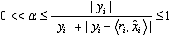
LabVIEW was used to implement the compressive data acquisition algorithm because of its graphical and interactive programming capabilities. The main LabVIEW program is shown in Fig. 2.
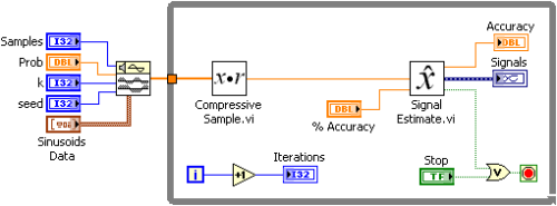
Fig. 2. High-level LabVIEW block diagram
The Compressive Sample VI shown in Fig. 3 is simply the dot product of the input Signal and the generated Random Sampling Basis.
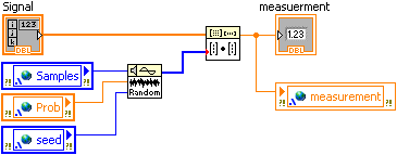
Fig. 3. Random sample (measurement) program
The Estimate Signal subroutine implements equation (7) using the Discrete Fourier Transform as the corresponding transform operation T{•}. Analysis of the LabVIEW block diagram in Fig. 4 shows the signal flow representation to obtain an estimate of x.
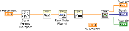
Fig. 4. LabVIEW block diagram to reconstruct the signal
Fig. 5 shows the results of running the LabVIEW program shown in Fig. 2 using Samples = 4096 (N), %Accuracy = 99 (α), Prob = 0.1 and k = 7.
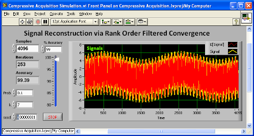
Fig. 5. LabVIEW front panel results
The simulation results show that for this particular set of parameters, it took 253 iterations (measurements) to reconstruct a wideband signal consisting of k sinusoids with approximate accuracy of 99.39%. Since this simulation is interactive, the iterations required to reconstruct vary. In this simulation we observed iterations in the 200 - 700 range.
Fig. 6 shows a zoomed portion of the signal where the yellow curve is the original signal and the red curve is the reconstructed signal using the rank order filtered convergence algorithm.
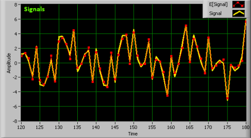
Fig. 6. Zoomed in results to show the original signal (yellow) and the signal reconstruction details (red).
1. Download and unzip the comp_daq.zip file
2. Open the Compressive Acquisition.lvproj LabVIEW project file
3. Open the Compressive Acquisition Simulation.vi
4. Configure the following controls on the front panel:
5. Run the VI
6. See the results on the front panel
LabVIEW 2009 or compatible
N/A
Additional Information or References
[1] Compressive Sensing Resources, http://www.dsp.ece.rice.edu/cs, Rice University.
Eduardo "Lalo" Pérez, Ph.D. was born in Mexico City, Mexico and obtained a B.S. E.C.E in telecommunications in 1981, M.S. E.C.E in image processing in 1983 and Ph.D. E.C.E. in real-time image processing in 1989 all from The University of Texas at Austin, Austin, TX, USA. Dr. Eduardo "Lalo" Pérez first joined National Instruments in 1985 while completing his Ph.D. and is one of the original members of the LabVIEW development team where he was responsible for designing and implementing the Digital Signal Processing and Data Analysis Libraries, still being used today. Dr. Pérez has over 20 years of industrial experience in the areas of real-time multiprocessor programming for the deployment of audio-visual telecommunications. Lalo has extensive experience in large enterprises - where he successfully deployed global multimedia networks and services for AT&T and Ernst & Young - as well as startups where he forged strategic alliances with Intel, Microsoft, Samsung and Texas Instruments to accelerate adoption of audio-visual services over IP.
**This document has been updated to meet the current required format for the NI Code Exchange.**
Example code from the Example Code Exchange in the NI Community is licensed with the MIT license.
Lalo, this is a great document! Thanks for adding it. I noticed that the last image is missing...
Todd,
Thanks for your comment. As you can see, I have updated the page to show the missing images.
Most importantly, I hope this sparks interest from the signal processing and DAQ communities.
-- Lalo
This tutorial was highlighted on the compressive sensing blog, Nuit Blanche. Check it out!
-Hilary
Dear Lalo,
Thanks for the example. I have a question for you with regards to the reconstruction algorithm, can you please contact me by E-mail ?
Cheers,
Igor.
http://nuit-blanche.blogspot.com
Dear Lalo,
Thank you for example. This project is the first VI abount Compressive sensing. Now I am try to compress and reconstruct a image with compressive sensing theory. I am wondering whether you have done some work on image compressive sensing or not. And I have found the reconstrution algorithm you used must know the sparisity of signal. Is that correct?
Dear Lalo Perez
Thank you for your explain about CS using LabVIEW.
That is very helpful to me to understand about CS. (Most CS coded MATLAB).
Anyway, I'd appreciate it, if you could explain how to induced formula (6) from (2) ?
Best Regards.
Jeong.
