- Document History
- Subscribe to RSS Feed
- Mark as New
- Mark as Read
- Bookmark
- Subscribe
- Printer Friendly Page
- Report to a Moderator
- Subscribe to RSS Feed
- Mark as New
- Mark as Read
- Bookmark
- Subscribe
- Printer Friendly Page
- Report to a Moderator
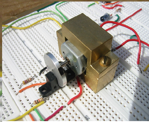
Figure 1: Tachometer apparatus to measure motor speed
The ability to translate electrical signals into motion in the real world combined with the ability to measure position can help you exploit the power of the computer to generate computer automation − the source of much of the modern world’s conveniences.
Purpose:
In this experiment, use the power capacity of the NI ELVIS II variable power supply to run and control the speed of a small DC motor. Using a modified free space IR link, build a tachometer to measure the speed of the motor. By combining the motor and tachometer with a LabVIEW program, you can incorporate computer automation in the system.
Equipment:
- 1 kresistor (brown, black, red)
- 10 kresistor (brown, black, orange)
- IR LED/phototransistor module OR an IR LED and a separate Phototransistor
- DC motor
- Small punch or drill
- Glue
- NI ELVIS II Series or myDAQ
- Optional: Several combs with varying numbers of teeth per inch
*Note: If you are implementing this project with the myDAQ, instead of using a variable power supply (VPS), use the myDAQ's Analog Output to set the voltage.
Set Up Hardware:
Hooking Up The Motor
You can purchase a small, inexpensive DC motor at Radio Shack or many hobby stores. These motors usually require a voltage source from 0 to 12 V, and produce a maximum RPM of about 15,000 at 12 V. With no load, the current requirement is usually about 300 mA. The NI ELVIS II VPS can supply up to 500 mA at 12 V. Also, by changing the polarity of the applied voltage, you can change the direction of rotation.
Complete the following steps to install and run a motor on an NI ELVIS II protoboard.
1. Connect a DC motor to the VPS output terminals, (SUPPLY+ and GROUND).
2. Launch the NI ELVIS II Instrument Launcher strip and
select Variable Power Supply (VPS).
3. From either the workstation’s manual VPS controls or the SFP controls, test the motor.
Note: It is a good idea to look up the specifications of the motor being used, if they are not already known, to make sure that too great of a load is not applied to it.
In the following example, manual control has been selected by clicking on the Manual box []. Read the VPS voltage by clicking on the Measure Supply Outputs box [], applying power to the protoboard, and clicking Run.
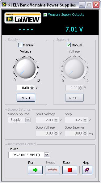
Figure 2: VPS supply configured to manually drive a DC motor
The Tachometer
Using an IR LED and phototransistor or an integrated LED/phototransistor module, you can build a simple motion sensor.
Complete the following steps to build a simple motion sensor:
1. On the protoboard, insert the components shown in the Figure 10.2 circuit diagram.
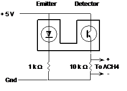
Figure 3: Circuit for operation of an integrated LED/phototransistor module
2. In the case of an LED/phototransistor module, an internal LED is used for the optical source. Power it from the +5 V power supply through a 1 kcurrent limiting resistor Then connect a 10 kW resistor from the phototransistor emitter to ground and connect the same +5 V power supply to the phototransistor collector. The voltage developed across the 10 kW resistor is the phototransistor or tachometer signal.
3. Connect leads from the 10 kresistor to the AI 0+ and AI 0- pin sockets.
4. Select Scope from the NI ELVIS Instrument Launcher strip and select the settings, as shown in Figure 4.
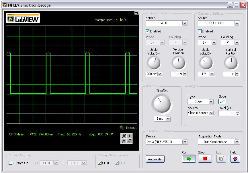
Figure 4: Tachometer signal viewed on the Oscilloscope
5. Power on the protoboard and run the oscilloscope SFP.
6. Pass a piece of paper through the IR motion sensor. You should see the oscilloscope trace change (HI-LO-HI). With a narrow piece of paper, you might catch the pulse generated as you drag it through the sensor.
Optional: Place a comb with many teeth in the sensor IR beam. Dragging it through the sensor generates a train of pulses. You can even run it back and forth like a saw to generate a continuous stream of pulses as shown in Figure 4.
It is interesting to try combs with different sizes and numbers of teeth. Each comb generates its own signature waveform.
Building a Rotary Motion System
The rotary motion demonstration system consists of the DC motor controlled by the variable power supply and the IR motion sensor configured as a tachometer. To complete the tachometer, you must attach a disk with a 2 in. diameter, to the shaft of the motor by completing the following steps.
1. Cut a 2 in. diameter disk from a piece of thin but sturdy cardboard or plastic.
2. Cut a slot about 0.25 in. wide and 0.25 in. deep near the circumference of the disk.
3. Punch or drill a small hole at the center point.
4. Glue the disk to the end of the motor shaft.
5. Mount the motor so that the slot lines up with the IR transmitter/receiver beam. In operation, each revolution generates one pulse.
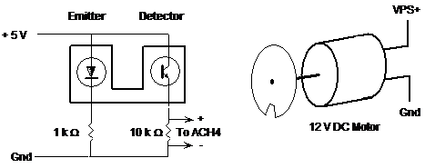
Figure 5: Motion sensor circuit and motor parts
Note: You can also use the CD and motor of Lab 6. Instead of a small magnet triggering the sensor, you can drill a hole about the size of the transmitter/receiver beam (3 mm) near the edge of the CD. Align the IR sensor so that the beam passes through the hole.

Figure 6. Apparatus to measure the speed of a spinning CD
Testing the Rotary Motion System
Complete the following steps to test the rotary motion system.
1. Power on the protoboard and run the motor using the NI ELVIS II VPS SFP to control the motor speed.
2. Adjust the motor position so that the disk does not touch the sensor slot.
3. Observe on the oscilloscope the pulses generated by the rotating motor, as shown in Figure 7.

Figure 7: Typical tachometer waveform
4. Read the pulse frequency (Freq:) from the measurement row CHO Meas: at the bottom of the oscilloscope screen. Take frequency measurements for a variety of power supply levels. A plot of frequency versus VPS voltage level demonstrates the linearity of your rotary motion system.
5. Close NI ELVIS and all SFPs.
Software Instructions:
A LabVIEW Measurement of RPM
LabVIEW has several VIs located at Functions»Programming»Analog Waveform»Waveform Measurements that are convenient for measuring the timing periods of a continuous waveform. You can use the Pulse Measurements.vi to measure the period, pulse duration, or duty cycle from a waveform array.
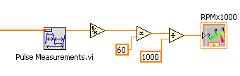
Figure 8: Period measurement converted to kRPM
You can convert the period measurement to revolutions per minute by inverting the period to get frequency and multiplying by 60 to get rpm. For scaling, divide by 1000 to get krpm.
Note: You can also use the Express template for Timing and Transitions Measurements and get the frequency directly. Then convert the frequency to rpm as discussed above.
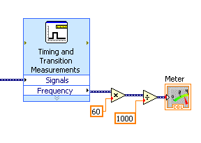
Figure 9: kRPM measurements using an Express VI
Using LabVIEW, complete the following steps to measure the period/frequency on a continuous waveform.
1. Launch LabVIEW and open RPM.vi from the Hands-On-NI ELVIS II library folder.
2. Open the diagram window and study the program.
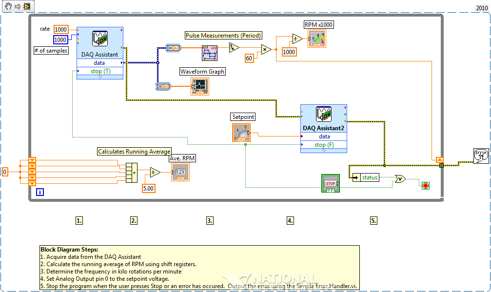
Figure 10: Block diagram of program RPM.vi
3. Before the vi can run properly, the express vi’s have to be linked to the correct channels on the Elvis being used. Double click on the “DAQ Assistant.” Next, right click where “Voltage” is highlighted and select “Change Physical Channel…” Navigate the menu and select the proper analog input channel. Double click on the NI ELVISmx Variable Power Supplies vi. Select your device from the drop down menu under instrument control.
Use the DAQ Assistant to collect 1000 V samples for the tachometer graph and provide an input signal array for the Pulse Measurements.vi. The rpm signal is sent to a front panel meter and displayed in krpm. The rpm signal also goes to a shift register with five elements. This provides an averaged rpm signal for the front panel. You manually control the motor speed with the front panel knob labeled Setpoint. Also available on the front panel is a graph of the tachometer signal as a function of time.
Run this VI and take your motor for a spin. See and hear how responsive the motor is to a rapid change in the rpm setpoint.
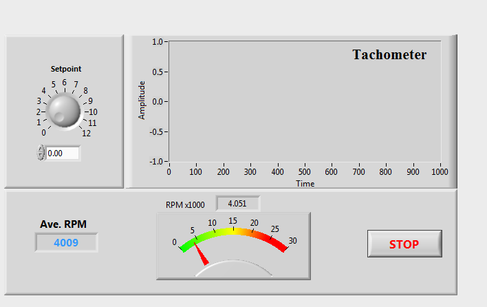
Figure 11: LabVIEW tachometer and motor control circuit front panel
LabVIEW Challenge: Computer Automation of the Rotary Motion System
National Instruments offers the LabVIEW PID Control Toolkit, which features additional LabVIEW VIs you can use to add computer automation to your rotary system. PID stands for “proportional integral derivative.” These control algorithms move a system from one setpoint (initial rpm) to another setpoint (final rpm) in an optimized manner. The addition of a single VI (PID.vi) provides optimal control to your program. The algorithm compares the target rpm (final rpm) with the current rpm (averaged rpm signal) to generate a DC error signal, which drives the VPS. Integration and differentiation parameters adjust the VPS voltage smoothly from one measurement to the next.
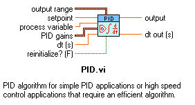
Figure 12: PID subVI for control applications
If you are more familiar with control, you can use another VI (PID Autotuning.vi) to set the initial PID parameters automatically. Then you can fine-tune the parameters to your specific system. Search for additional LabVIEW PID resources at http://www.ni.com.
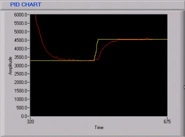
Figure 13: Setpoint (yellow) and RPM (red) traces show optimal control PID in action
In Figure 13, the setpoint (yellow trace) is changed suddenly from 3300 to 4500 krpm. The system rpm (red trace) responds by moving the motor speed smoothly and optimally from the current setpoint to the target setpoint.
