Simultaneous Fiber-Optic Chronoabsorptometry / Chronoamperometry: Data Collection

[roadchem]

Overview

This vi collects chronoamperometry data and chronoabsorptometry data simultaneously to yield quantitative spectroelectrochemical data in the form of absorptivity (extinction coefficient) vs. wavelength plots.  A correction for edge-diffusion can be applied to the chronoamperometry data which is then integrated to yield charge vs. time data.  From the integrated data, charge values are assigned to each spectrum collected.  The program does a least-squares analysis of the absorbance vs. charge data at each wavelength, and with some additional input will yield the absorptivity vs. wavelength plot of the electrode product.

The data can be later re-analyzed using one of two other packages available on the NI site, depending on whether there is a kinetically-important intermediate (or not).   Detailed documentation is provided within each vi and in the readme.txt file included in the zip file.  This procedure is described in detail in an upcoming issue of Inorganic Chemistry (reference: Inorg. Chem., Article ASAP, DOI: 10.1021/ic1012654, Publication Date (Web): September 13, 2010).

To be absolutely clear, this vi calculates absorptivity or extinction coefficient from absorbance data and charge data which are collected simultaneously over time during a chronoamperometry experiment.  Absorptivity, e, is related to absorbance via Beer's Law A=ebc where b is path length (cm) and c is concentration (M).  When the term "spectrum" is used herein, I specifically mean an e vs. wavelength plot.

Caveats and Additional Notes

 The suite of programs was originally designed for a Princeton Applied Research Potentiostat interfaced by a GPIB connection (device 14) to a PC which also has an NI-USB 6251.  An analog potentiostat will work fine with slight modifications to the program which remove the GPIB functions.

The hardware is set up as follows:

1. An analog output from a NI-USB 6251 is attached to the external input of the potentiostat and it controls the potential applied to the cell.
2. A pair of analog input channels (run as one task) records the applied potential and applied current from the potentiostat's E-output and I-output respectively.
3. A digital output channel from the 6251 is attached to the trigger input of an Ocean Optics USB-4000 fiber-optic spectrometer, and the spectrometer's software is configured to automatically record spectra upon receiving trigger signals (specifics are in the readme.txt file.)  This application does not use the Labview Ocean Optics driver.
4. In a typical run, the current which passes through the electrode as a result of a potential step is recorded (chronoamperometry) while spectra of the solution at the electrode surface are recorded simultaneously (chronoabsorptometry).  We usually record 20 spectra over a 10-second period, but we have pushed it down to 10 spectra over 2 seconds.
5. The cell design uses a bright source like an LS-50 Ocean Optics Tungsten Lamp, a "dip probe" from which the mirror has been removed, and the USB 4000 detector.  The dip probe is positioned so that its light shines on and is reflected from something like a 3 mm Pt disk electrode.  It is important to have enough signal so that a spectrum can be collected in less than 15 milliseconds, and careful alignment is required.  It is also important to stir or agitate the solution between scans.  Details of a cell used for this purpose have been published.

Detailed description:

This set of vi's is used to collect and do some initial processing of simultaneous chronoabsorptometry / chronoamperometry data.  A pair of separate packages are provided for further data processing depending on whether or not there is a detectable intermediate present.  The data collected by this vi can be used to determine the spectra of electrode products.  Two cases have been developed so far:

1. A separate program can be used to collect absorptivity vs. wavelength information about a single electrode product for a 100% chemically reversible or 100% chemically irreversible electrode reaction.
2. A similar but again, separate set of data analysis vi's is available for the case of an electrode reaction which involves an intermediate which decays into a final product by a first or pseudo-first order process.  Basically, if cyclic voltammetry can detect the process at scan rates of 500 mV/s or less, the spectrum of the intermediate and the product can be obtained.  Some smoothing may be required.

The end result of this approach is absorptivity vs. wavelength data for electrode products.  This approach is based on equations developed to remove any arbitrary interactive spectral subtraction of the starting material from difference data.  This quantitative approach yields absorptivity information which is often lacking in other spectroelectrochemical methods, and provides information on the same timescale employed by cyclic voltammetry.

The method:

The specifics of the method have been described elsewhere (currently in press in the journal Inorganic Chemistry).  The general functions of the data collection program are:

1. The technique uses a fiber-optic spectrometer to take light to and from an electrode surface.  Labview controls a potentiostat to apply a chronoamperometry waveform, to trigger the spectrometer, and to record potential-current-time data from the spectrometer.
2. The vi integrates the current and figures out how much charge has been passed through the electrode at each point in time when a spectrum is recorded.  An optional edge correction can be applied which corrects for edge-diffusion... to take advantage of this feature you need to have measured the diffusion coefficient of the starting material and the physical radius of your electrode.  The chronoamperometry vi's previously posted on the National Instruments site  [Chronoamperometry Data Collection and Basic Analysis by Mike Shaw] can help.
3. The set of spectra and the charges are processed by a least squares plot of absorbance vs. charge at each wavelength to yield a "change in absorptivity vs. wavelength" plot.  If a spectrum of the starting material at known concentration and pathlength is available, and if the electrode area is known, then the absorptivity vs. wavelength plot of the electrode product is saved.

Spectrometer setup:

The spectrometer software must be configures separately.  We have used Ocean Optics spectrometers with their OOIBase or Spectrasuite programs.  The vi is configured to read "tab-delimited ascii files with header" and the filenames should be set to autoincrement.  The filenames should be of the format "filename.00001.abs" and should be absorbance files.

We usually use a bright source such as a tungsten lamp (e.g. LS-50 from Ocean Optics) which gives strong signals in the 380-950 nm range so that a good spectrum can be obtained in less than 15 milliseconds.  We take a dark spectrum, and then a reference spectrum and set the software to absorbance mode.  The technique relies on difference data so it is OK to take a reference spectrum with the sample present.

The trigger is then set to the software setting.  Then the file saving options are set to record every spectrum, the filename is set to the proper format (above... put a period after your filename like "filename." and set to autoincrement), the file type is set to ASCII tab delimited with header.  Put your new files in a new directory.  It might be a good idea to set the maximum number of files recorded to a value like 1000, so that if you make a mistake, the harddrive does not get filled with useless spectra.

Spectrasuite will be unresponsive while it is waiting for a trigger signal.  When you are done with it, or need to change something, I would close the program (it won't close completely until you send a trigger signal), and use the Measurement and Automation Explorer to send a trigger signal which will close the program.

Absorbance file format

1. File format should be tab-delimited text file generated by Ocean Optics OOIBase or Spectrasuite program. The wavelength vs. absorbance pairs should begin on the 18th line.  The last line should read:  >>>>>End Processed Spectral Data<<<<<
2. The files should be named according to name.XXXXX.txt.  In Spectrasuite, this can be accomplished automatically when setting up the files to be automatically recorded in a directory on the software trigger setting.  Note that the period before and after the XXXXX is important, as A_vs_Q.vi strips
   the text before and after the periods so as to come up with a set of numbers, each of which corresponds to a spectrum which is read into a separate array.
3. Examples of files are included.
4. Data and Spectrocoulometry_data_workup.vi program courtesy of M. Shaw, Department of Chemistry, SIUE.  All vi's are provided "as-is" with no expectation or implication of warranty or troubleshooting.

Description of vi's:

The main vi is called  "Data_Collection_amperometry_absorptometry.vi".  When it runs, there is a pause at the beginning so that the user can double check if the setup is correct, and also to decide whether or not to run the edge correction vi.  During initial data collection, it is recommended that the edge correction not be used.  When all the sub-vi's have run, the result is displayed on the front panel of this vi.

Here is a screenshot of the block diagram:

The first frame (not shown) simply allows for a pause so the user can make sure the cell is on, has been stirred, and everything else is ready.  The overall program calls subvi's as follows:

1.  VIS_NIR_PULSE3.vi collects simultaneous chronoamperometry/chronoabsorptometry data
2.  The user can choose to do an edge correction or not.  Probably best not to bother during the experiment
     Better to do edge correction after all the data has been collected in a separate data analysis step... use the
     "Data Workup" vi's provided separately.
3.  A vs Q.vi performs least squares analysis of absorbance vs. charge data at each wavelength... can provide
    a difference spectrum, or with some more information, the actual absorptivity vs. wavelength plot of the
    electrode product.
4.  Displays the final spectra information on the front panel as an XY graph.

After the program is complete, I would make sure that all the files that correspond to a single run are collected in a single directory. That may mean moving the spectral files which were collected by Spectrasuite into the same directory where you saved the potential-current-time data and also the final absorptivity vs. wavelength data.  I usually create a directory using the current date, and create a bunch of subdirectories called "attempt1", "attempt2", "attempt3" etc in addition to a directory called "spectra" where Spectrasuite can deposit the data files it collects.  After each experiment I make sure the data files are collected together because it is usually very difficult to disentangle them at the end.

Between each run you must stir the sample to make sure the solution at the electrode is fresh.

The sub-vi's run as follows:

(1) "VIS_NIR_PULSE3.vi"allows the user to set up a double-potential-step chronoamperometry experiment where the electrode starts out at some rest potential, applies the waveform, and then returns to the rest potential.  Here is a screenshot of the front panel:

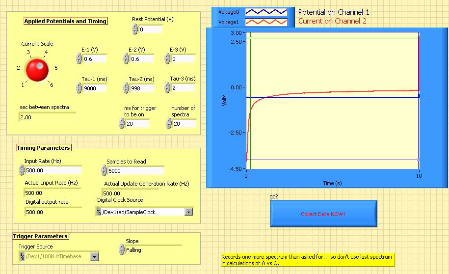
The "rest potential should be set to a value where no current flows through the electrode (not always "zero").  It is best to have the final potential (E-3) be the same as the rest potential for 2 milliseconds.  The other two potentials should be set to the same value for the balance of the time.  In the example above, the entire experiment is set for 10 seconds total, but one could change that to 2 seconds by making "Tau-1" be 1000 ms.  The total time needs to be the same as "Samples to read" divided by "input rate".  The vi assumes that the potentiostat is a Princeton Applied Research instrument (e.g. PAR 273A or 263A or Versastat II) connected via GPIB at address 14.  If not, the vi will still work, but the rest potential will be stuck at zero.

The user should set the current range sensitivity setting so that current-overloads don't happen.  For a 3mm Pt disk electrode with a 1 mM solution of ferrocene in 0.1M NBu4PF6/CH2Cl2, a setting of -4 works well.  This setting corresponds to full scale on the potentiostat being 1E-4 amps per volt measured (~2V max).  For lower concentrations, a more sensitive setting (i.e. "-5") might be required.

Once all the parameters have been set up for the experiment, the user will click on the "collect data NOW" button.  The vi will set up the PAR potentiostat via GPIB to apply the external potential supplied through the external input from the NI-6251 board, then it will apply the potential.  It will measure the potential and current reported by the potentiostat via the external outputs while sending a series of trigger signals to the spectrometer to measure spectra.

This vi then saves the time, potential and current data in a tab delimited spreadsheet file which the user specifies via a dialogue box which opens after data collection.  It is a good idea to enter the filename within a single minute after the dialogue box opens, otherwise the potentiostat might hang.  If this happens, just shut off the potentiostat and turn it back on again.

The measured current and potential will briefly be displayed and then the vi will close as the next subvi executes.

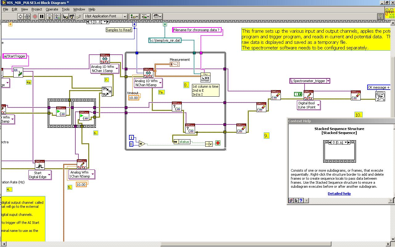
The block diagram consists of a stacked sequence structure with 8 frames, each of which has comments explaining the various functions. To summarize:

Frame 0:  Sets up a PAR potentiostat at address 14 to apply externally supplied potentials with the cell on and to not autorange.

Frame 1:  Sets up potentiostat's current scale.

Frame 2:  Sets up potentiostat's rest potential.

Frame 3:  Takes the "Tau times" the potentials, the data collection rate, and the number of samples, and generates a waveform which corresponds to chronoamperometry.

Frame 4: Sets up the various input and output channels, applies the potential program and trigger program, and reads in current and potential data.  The raw data is  displayed and saved as a temporary file.  The spectrometer software needs to be configured separately.  There is extensive notation on this frame.  Users will need to make sure their DAQmx task names are configured and named correctly.  I have used "E and I output" to measure the potentials on two analog input channels,  "Spectrometer_trigger" for a digital output, and "Applied_E" as the analogue output which is connected to the external input of the potentiostat.  This vi is a modification of an I/O application provided with Labview and is similar to what is used in my "Cyclic Voltammetry with an analogue potentiostat" example.  The user will need to make sure  that the tasks configured are set up right.  There is a digital output for the trigger signal to the spectrometer, an analog output to control the potential applied by the potentiostat, and a task which comprises two analog inputs from the potential and current outputs of the potentiostat, respectively.

The final waveform data is saved as a temporary file after data collection when a dialogue box opens which asks the user for a filename.

You will need a c:\temp directory.

Here are left and right side screen shots of the frame

Frame 5:  This frame opens the temporary file, and integrates the current and picks out the charge values which correspond to times at which spectra were recorded. These charges are passed on to the next vi.

Frame 6:  This frame completes the conversionof current to amps and saves the time-potential-current data in its final form as a spreadsheet file.

Frame 7:  Turns the cell off and deletes the temporary file from c:\temp

The vi usually collects an extra spectrum, so ignore the last spectral file when processing.

"VIS_NIR_PULSE3.vi" calls a couple of other sub vi's:

(A)  "Get Terminal Name with Device Prefix.vi" is included here, although it is also found in:  C:\Program Files\National Instruments\LabVIEW 8.2\examples\DAQmx\_Utility\_Utility.llb or the equivalent library in your machine.

(B)  "Ocean_Optics_Trigger_Signal.vi" constructs a digital waveform to control when the trigger signal is sent to the Ocean Optics Spectrometer.  It uses the total time allottedfor the scan and the scan rate to build an array of "on" signals, and substitutes the "off" times into the array based on how many spectra are to be recorded, and how long (in milliseconds) the trigger signal needs to be on for.  The array is then converted into the waveform used in the main program.

(C)  Similarly, "pulse waveform generator.vi" takes a resting potential, three applied potentials and three times (tau) which to apply each potential and constructs an analog waveform appropriate for double potential step chronoamperometry.  This vi thus has flexibility for future applications (such as a cyclic absorptometry application currently being developed) .  These values are fed to this vi from the front panel of "VIS_NIR_PULSE3.vi", but this vi could be used on its own for double potential step chronoamperometry with minor modification (e.g. removing the spectrometer trigger stuff).

(2) The "Edge_correction.vi" program applies a correction to the chronoamperometry data to yield the charges that correspond to each spectrum recorded.  For small electrodes, edge diffusion can result in a systematic and increasing error in the charge obtained when current vs. time data is integrates, as described by Heinze.  This vi is optional during data collection, but should be applied when the final data analysis is underway.  It requires the diffusion coefficient of the starting material which can be obtained from a separate chronoamperometry experiment.  This vi has been described in detail in a separate document called "Chronoamperometry Correction for Radial Diffusion: Chronocoulometry" .

(3) The  "A_vs_Q.vi" performs a linear least squares analysis of the absorbance vs. charge data at each wavelength.  The user can choose between a difference spectrum format, and the actual absorptivity of the product vs. wavelength plot.  For the latter you will need a spectrum of the starting material at known concentration and path length, as well as the electrode area (as determined by chronoamperometry) and the diffusion coefficient of the analyte... I usually just look at the difference spectrum and wait until later to process the data.  This vi saves the final spectrum as a spreadsheet file.  The various columns are wavelength, absorptivity, and relative standard deviation.

Here is a screenshot of the front panel:

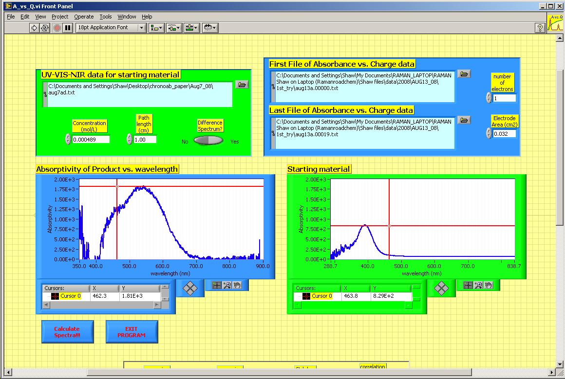
During data collection, I would:

1. Enter the filename for the starting material's UV-VIS-NIR data (tab delimited file from Spectrasuite) in the green box.
2. Enter the starting material's concentration and path length in the green box.
3. Decide whether you want a difference spectrum (change in absorptivity), or the absolute absorptivity vs wavelength graph. I strongly suggest a difference spectrum.  If you select to do a difference spectrum, then the path length and concentration become irrelevant, and you just need any valid spectrum's path entered in the green box.  This is useful if you have not yet measured the spectrum of your starting material.  The path length to enter in the green box is NOT the path length you have during the spectro-e-chem experiment (which is mathematically irrelevant) but the path length of the sample you measured your starting material's spectrum with.
4. In the blue box, you need to enter the spectra data you just collected.  The upper path box is for the first spectrum, and the lower path box is for the final spectrum.  As described under "Spectrometer setup" your files will have names similar to "sample.00XXX.abs" where the "XXX" corresponds to the number of the spectrum automatically saved upon the spectrometer's receipt of the trigger signal.  There may be one extra spectrum collected, so make sure you enter in the same number of spectra as you requested in the data collection vi.
5. Click on "Calculate Spectrum" and the green XY graph will just display the absorptivity (from Beer's law, your starting material's spectrum, path length, and concentration), while the blue graph will display the change in absorptivity that occurs at the electrode surface due to the consumption of starting material and formation of product. Ideally, the spectrum of the product is just the difference spectrum added to the spectrum of the starting material (by spectrum I mean absorptivity vs. wavelength plot).
6. The program will ask you for a filename and it will save your absorptivity vs. wavelength file where you specify.
7. You can return to the main front panel display by clicking on "exit program."  Alternately, you can click on the stop button, make adjustments to your parameters and run the sub-vi again until you are satisfied.

The block diagram consists of a stacked sequence structure with 3 frames.

Frame 0:  Pauses the program until the filenames and other data have been entered correctly.

Frame 1:  Prompts the user for a filename for the final absorptivity vs. wavelength file

Frame 2:  This frame does a lot....

(1)  Loads the spectra into an array.
(2)  Performs a least squares analysis of Absorbance vs. Charge at each wavelength. 
(3)  Calculates starting material absorptivity data from a representative spectrum recorded at known concentration and known pathlength.
(4)  Calculates the absorptivity of the product.

Frame 3: Pauses the program while the user inspects the graphs.

Here is a screenshot of part of Frame 2:

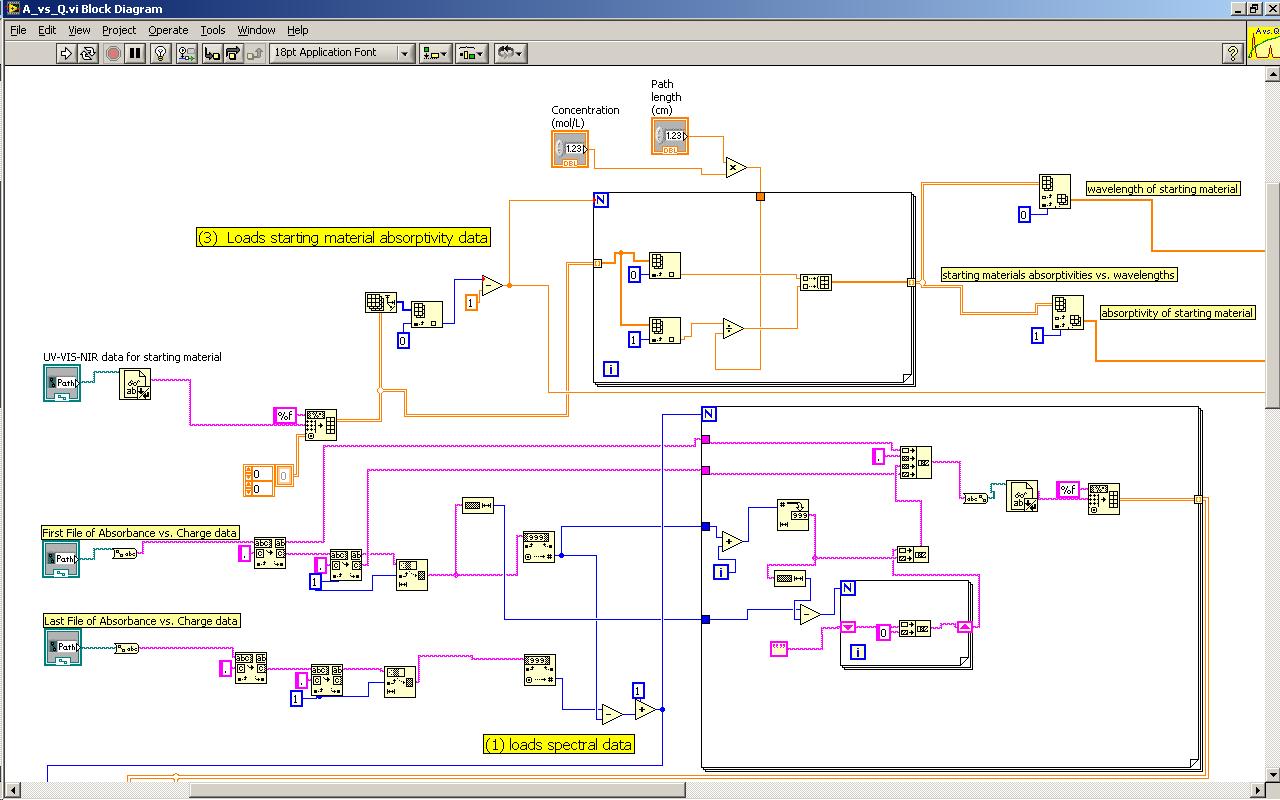
This part of Frame 2 (above) loads the starting material's spectrum into an array.  It also loads all of the spectra between (and including) the first and last spectra

specified by the user into another single array.

This part of Frame 2 (above) performs a least squares analysis at every wavelength (Y-values) vs. the charge (X-values) for the arrayed spectra.  There will be one charge which corresponds to each spectrum.  In a usual run, there are about 2000 wavelengths analyzed at each of these charges.  Ideally, charge increases with the square root of time.  While regression analysis is part of many versions of Labview, I programmed this function because the regression analysis is not part of every version of Labview.

In this part of Frame 2 (above), the starting material's spectrum, path length and concentration are converted in absorptivity.  There is a correction from the molarity units in Beer's law to the moles per mL units required for the Cottrell Equation.  The loop at the bottom of the frame translates the regression slopes at every wavelength into absorptivity values.  These arrays are then fed into XY graphs and the data is saved.

Steps to implement or execute code
To implement this example:

1. Run the VI

Requirements
Software
LabVIEW 2012 or compatible
NI-DAQmx 16.0 or compatible

Hardware
cDAQ with compatible C Sries

Previous and current (CHE 0911537) support by NSF is gratefully acknowledged for this work.