Chronoamperometry Correction for Radial Diffusion: Chronocoulometry
- Subscribe to RSS Feed
- Mark as New
- Mark as Read
- Bookmark
- Subscribe
- Printer Friendly Page
- Report to a Moderator
Code and Documents
Attachment
Functional Description
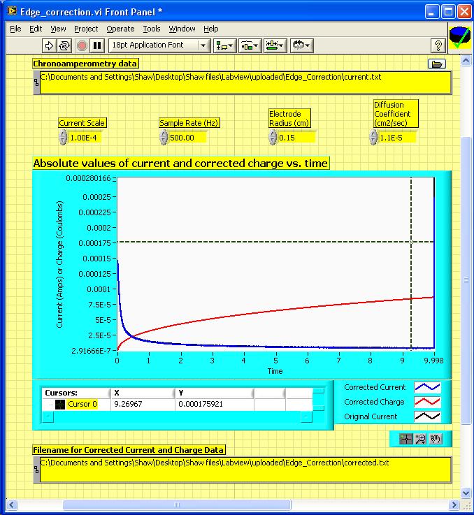
This vi takes data generated by the chronoamp_engine.vi in the chronoamperometry set of vi's posted previously, applies the edge correction for radial diffusion described by J. Heinze [1] and integrates the current to yield Chronocoulometry data (i.e. charge vs. time). The data is saved in a spreadsheet file and displayed in an XY graph. Here is the front panel:
Caveats and Additional Notes
The input file should be a tab-delimited spreadsheet file where the first column is time (seconds), the second column is potential, and the third column is current. A sample file is included (Current range: 1E-4 Amps/Volt). If the current is in amps, then a value of 1 can be entered into the current range setting. If the current is in milliamps, then a value of -3 should be entered into the current range setting. If the current is in microamps, then a value of -6 should be entered into the current range setting. The sample rate is frequency at which data was recorded.
These values should be set the same as for when the data was recorded, if the suite of chronoamperometry vi's I previously posted are used to collect the data.
The specific correction applied is that the current is divided by the factor
[1 + (eta)(b)] where
eta = {Dt/R^2)^.5
b = value from "table 1" [1] which was found by digital simulation.
D= diffusion coefficent of analyte
t = time
R = radius of electrode in cm as measured with a ruler (or calipers)
The plot of b vs. eta was fitted to a 5th order polynomial in an Excel spreadsheet (by me, not published except here), and a very good fit was found. Here is a screenshot of the block diagram:

If the diffusion coefficent of the compound is known and the electrode radius is known, then both eta and b can be found easily, and thus the edge correction can be computed.
Why would anyone do an edge correction in the first place?
The equations for chronoamperometry and chronocoulometry assume that analyte molecules diffuse to an electrode whose area is infinite, i.e. they all diffuse somewhere in the middle of the electrode from the z-direction. Real electrodes have a perimeter where diffusion can ALSO occur from the x and y direcions. This edge diffusion shows up as a larger-than-expected current. The smaller the electrode, the more problematic this effect is.
Fortunately, for most chronoamperometry experiments, edge correction is not necessary. This is because electrode areas and diffusion coefficents etc are calculated from the slope of Cottrell plots. The corrected and the uncorrected current data give virtually parallel lines in Cottrell plots, so the slopes are the same.
Where edge correction is necessary is for tiny electrodes. Edge correction is also necessary when you want to integrate chronoamperometry data to yield chronocoulometry data. Even "large" electrode areas of 1 cm-squared can benefit from the edge correction. The small differences in corrected and uncorrected chronoamperometry data are magnified upon integration and give poor Chronocoulometry data.
Chronocolometry is useful for determining the coverage of adsorbed materials on an electrode surface, either before or after electron-transfer.[2]
Previous and current (CHE 0911537) support by NSF is gratefully acknowledged for this work.
[1] J. Heinze J. Electroanal. Chem. 1981, 124, pp. 73-86.
[2] A.J. Bard, L. R. Faulkner "Electrochemical Methods: Fundamentals and Applications" 2nd Ed. Wiley, New York: 2001. See Chapter 5 for Chronoamperometry and Chronocoulometry.
Example code from the Example Code Exchange in the NI Community is licensed with the MIT license.
- Mark as Read
- Mark as New
- Bookmark
- Permalink
- Report to a Moderator
Thanks for posting! Could you please rename your attachment to include the LabVIEW version?
LabVIEW Community Manager
National Instruments
- Mark as Read
- Mark as New
- Bookmark
- Permalink
- Report to a Moderator
Done!
