- Document History
- Subscribe to RSS Feed
- Mark as New
- Mark as Read
- Bookmark
- Subscribe
- Printer Friendly Page
- Report to a Moderator
- Subscribe to RSS Feed
- Mark as New
- Mark as Read
- Bookmark
- Subscribe
- Printer Friendly Page
- Report to a Moderator
3D Orbital Tracking Microscopy
Contact Information
Competition Year: 2016
University: Ludwigs-Maximilian Universität München
Team Members: Fabian Wehnekamp
Faculty Advisers: Prof. Don C. Lamb
Email Address: fawepc@cup.lmu.de
Submission Language: English
Project Information:
Title: 3D Real-Time Orbital Tracking Microscopy
Description:
A microscope system to locate the 3D position of nanoparticles moving in tissue, cells or living animals with nanometer precision in real-time. In addition the microscope system records simultaneously informations about the environment.
Products:
NI Hardware:
NI cRIO 9082
NI 9263 Analogue Output Module x1
NI 9402 Digitoal I/O Module x3
NI PCI 6733
NI Software:
Labview 2015
Labview Realtime
Labview FPGA
Labview DAQ
Labview IMAQ
Labview Mathscript
3rd Party Hardware:
Scan IM Microstage (Märzhäuser Wetzlar)
zPiezo (Piezosystems Jena)
3D Piezostage (Physik Instrumente)
Ixon Ultra EMCCD Camera (Andor)
Galvanometer Mirros (Cambridge Technologies)
Avalanche Photo Diodes (Perkin Elmer & Laser Components)
405 nm Laser (Cobolt)
488 nm Laser (Coherent)
561 nm Laser (Cobolt)
633 nm Laser (Melles Griot)
Acousto optical tunable filter (Gooch & Housego)
The Challenge:
Life depends on the shuffling, transport and relocation of proteins on the cellular level. Several diseases can be linked to impaired transport processes, for example alzheimer, dementia or ALS. To reveal the underlying principles of these processes, we need the ability to record three dimensional trajectories of particles in their natural environment with a temporal resolution of a few milliseconds and a spatial resolution of a few nanometer. To achieve this all microscope components need to be synchronized on the microsecond timescale to be able to deterministically track a particle.
The Solution:
1. Orbital tracking concept:
The concept of orbital tracking microscopy relies on the modulation of the fluorescent signal during a full rotation of a laser beam around a fluorescent particle. This modulation can be used to determine the relative position of the particle to the center of this full rotation. To record a full trajectory of the particle, the center of the orbit has to be continuously updated to follow the particle after every step.
![]()
Fig. 1 | Orbital tracking principle
(Fig. 1a) The laser focus is rotated around a particle in the xy plane. Depending on the relative lateral position of the particle in relation to the center of the orbit, different modulations of the fluorescent signal can be observed. (Fig. 1b) For the axial particle localization, the fluorescence signal is detected slightly above and below the focus point of the objective. Depending on the axial position of the particle in relation to the focus, the ratio of the signal between the two avalanche photo diodes (APD) changes. The intensity values over a full orbit (16 detections points) can be described by a Fourier series:

The zero order coefficient describes the average intensity over the full rotation, whereas the first order coefficients encode the angular position of the particle in relation to the x axis and the distance to the center of the orbit. The position of the particle in relation to the center of the orbit can thus be described by:
![]()
z localization is performed through the intensity ratio between the two detection planes. The particle’s axial position in relation to the focal plane dz is given as:
![]()
To minimize the calculation time, both scaling functions, f(r) and g(z), are implemented with a combination of a look-up table and a binary search, which ensures a rapid determination of the new orbit position. Both look-up tables are generated prior to the experiment through simulations. After each calculation, the center of the orbit is moved to the current location of the particle and the feedback loop starts again.
2. Microscope Design
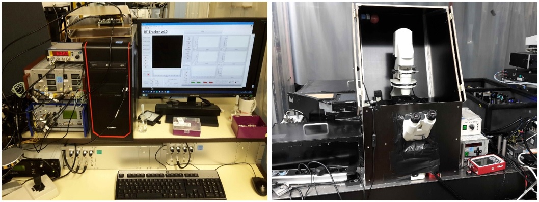
Fig. 2a | Microscope
(left) Microscope host computer and additional hardware control for z-piezo, avalanche photo diodes (APD’s), calibration piezo and acousto-optical tunable filters (AOTF). (right) Orbital tracking microscope: Microscope body, widefield microscope for environmental observation, confocal microscope for particle tracking and laser excitation module.
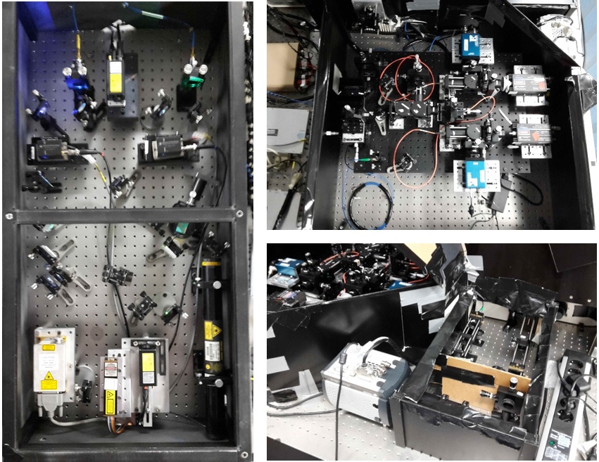
Fig. 2b | Microscope
(left) Laser excitation module: Combines 5 lasers (405nm, 488nm, 532nm, 561nm and 633 nm) and guides them via single mode fibers to the confocal microscope and the widefield microscope. Two acousto-optical tunable filters allow to enable different wavelengths and control the output power of each laser. (top right) Confocal microscope: two galvanometer mirrors control the lateral position of the laser beam. The fluorescent signal is detected by 2 detector pairs for green and red excitation. (bottom right) Widefield microscope: Records the environment of the tracked particle.
![]()
Fig. 2c | Microscope Schematic
3. Technical implementation:
Code structure:
The tracking algorithm is implemented with a combination of a normal computer as a front end for user interaction, data visualization and logging. Time critical tasks are performed on the NI compact RIO 9082 as deterministic back end.

Fig. 3 | Code structure
Host computer: Confocal state machine: Transfers user input to cRIO 9082, displays and logs data of the confocal microscope. Camera state machine: Transfers user input for camera to cRIO 9082 and reads out camera frames. Image state machine: Combines scanning images and camera image into an RGB image to display. Calibration state machine: Controls xyz calibration piezo.
Realtime computer: Confocal state machine: Controls confocal microscope, transfers data from FPGA to host. Camera state machine: Controls camera triggering.
FPGA: Confocal state machine: Analogue and digital I/O. Camera state machine: Triggers camera and counts frames.
Tracking feedback execution:
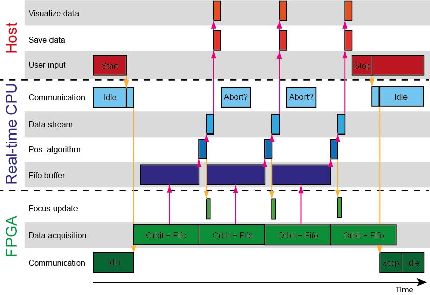
Fig. 4 | Tracking Feedback
The 3D tracking feedback is implemented through a combination of FPGA and realtime code. After the start command from the host computer, the FPGA starts to generate the orbit. After each orbit point the corresponding countrate is transferred to the realtime cpu via a DMA-FIFO. After all 16 elements per channel are read out, the new position is determined and is updated on the fly during the next orbit iteration. All parameters for each orbit are transferred via a network stream to the host computer. Depending on the operation mode of the tracking algorithm, several different modules are executed. The feedback loop is terminated by a user interaction.
User Interface:
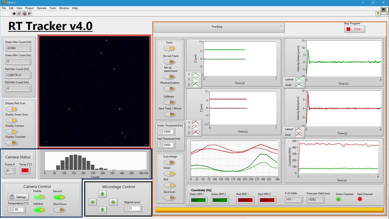 Fig. 5 | User Interface
The user interface is designed to give the user the optimal control over all microscope components and to display the real-time data generated from the cRIO 9082. (Red box) RGB image panel to display the combined data from the lateral scanning images of the confocal microscope and the image acquired through the IXON Ultra camera (red and green channel display confocal data, blue channel camera frames). (blue box) Controls and displays for the widefield microscope. The user is able to select different operation modes for the camera. While acquiring frames, the contrast range of the image can be manipulated through the countrate histogram. Acquired images can be recorded as tif-stacks. (black box) Control for the micrometer sample stage. During a measurement the stage control is performed through components of the tracking feedback loop. (Orange box) Controls and displays for the tracking microscope. Through the menu bar at the top different modes can be accessed (e.g. tracking mode, calibration modes and settings). Through the controls the user can perform lateral scanning images for different channels, set up experiment parameters and start the tracking of single particles. The waveform charts and graphs display the current position and velocity as well as the countrate and the orbit intensity data for up to two channels simultaneously. During the start of the program the user can select different measurement profiles which store the entered data upon closing the program.
Results:
System Performance:
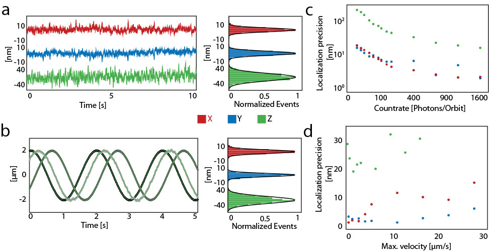
Fig. 6 | Orbital Tracking Precision
To measure the localization precision of the orbital tracking microscope, a sample containing 190nm fluorescent beads is used. (a) The localization of a stationary particle (190nm multifluorescent bead, Spherotech) at a countrate of > 1600 photons per orbit is shown as a function of time (acquisition rate 200Hz) for x, y and z in red, blue and green respectively. The localization precision, determined from the standard deviation of the position of the stationary particle, was ❤️ nm laterally and <21 nm axially. (b) Localization precision for a moving particle (with a maximum velocity of 6.2 μm/s). An immobilized particle was moved along a sinusoidal path using the xyz piezo stage and the position recorded as a function of time (acquisition rate, 200Hz) in x, y or z. A sinusoidal fit was performed (green lines) and the standard deviation of the residuals was used to determine the precision. For a count rate of > 1600 photons per orbit, a localization precision of < 3nm laterally and 21nm axially was measured. (c) Count-rate dependent localization precision (average values from stationary and dynamic particles, acquisition rate 200 Hz). The values for for x, y and z are shown in red, blue and green respectively. (d) Velocity dependent localization precision for a particle moving along the x, y and z axis. The decreased accuracy of the x axis compared to the y axis at velocities above 5 μm/s is a result of a ~0.1ms delay in updating the position of the particle at the starting point of the new orbit (ϕ=0°).
Tracking of individual mitochondria in zebrafish embryos:
Neurodegenerative diseases like Alzheimer, ALS and dementia can be linked to an impaired transport of mitochondria in nerve cells. Nerve cells consists of a cell body, the elongated stem axon and the peripheral arbor. Mitochondria have to be transported from the cell body to the arbor and backwards to ensure energy production at the arbor and to recycle damaged mitochondria. Although it is known that the impaired transport of mitochondria plays a role in neurodegenerative diseases, it is not clear how mitochondrial transport is regulated in a healthy nerve cell. To be able to resolve the individual details of transport, we need to use the high spatial and temporal resolution of the orbital tracking microscope. As a model system we are utilizing zebrafish embryos as a vertebrate model system, due to their easy handling and their optical transparent body.

Fig 7 | Tracking Mitochondria in Zebrafish embryos
(a) Zebrafish schematic with depicted measurement area at the tail of the fish. 2-3 embryos are embedded into an agarose gel and kept in embryo medium to maintain optimal conditions. To prevent the development of skin pigments which can impair the measurement, phenylthiourea is added to the medium. In addition, tricaine is used to put the embryo to sleep. When maintaining these conditions, the zebrafish can be kept for 24 hours in this agarose gel.
(b) Experimental setup schematic. The zebrafish embryos are put on top of the microscope and a properly developed neuron beard sensory neuron is selected with the widefield camera. By using 405 nm light a single mitochondrion can be “switched” on and tracked without being affected by other mitochondria. The individual mitochondria is tracked inside the stem axon until the fluorophores are completely bleached.
(c) Example trajectory of a single mitochondria moving through the stem axon of the nerve cell. With the orbital tracking technique we are able to follow a single mitochondria with a precision of ~5nm in xy and ~25nm in z over a distance of up to 100µm.
Video 1 | Tracking of a single mitochondrion inside a nerve cell
(left) Widefield movie of a moving mitochondria in a nerve cell inside a zebrafish embryo. White spots represent individual mitochondria. The faint white line the stem axon of the nerve cell. Trailing points indicate the trajectory of the moving mitochondria. The color coding indicates different types of transport processes. The visible shifts during the video are repositioning events during the tracking to avoid that the mitochondrion leaves the field of view of the camera. (top right) Photon count rate of the single mitochondrion. After 150 second the laser focus gets stuck on a brighter mitochondrion. The downward peaks represent repositioning events from the sample where the algorithm loses the mitochondrion for a short period of time. (bottom right) Two dimensional trajectory data of the mitochondrion from the widefield movie. The grey box indicates the field of view of the camera. The black box indicates the threshold level for a repositioning event. The grey bars along the trajectory represent stationary mitochondria inside the axon.
1.In vivo imaging of disease-related mitochondrial dynamics in a vertebrate model system. Journal of Neuroscience 32, 16203-12 (2012).
Benefits of Labview:
Our group is an interdisciplinary mixture of chemists, biologists and physicists which usually do not have any prior programming knowledge when starting a PhD. With the intuitive graphical programming approach it is very easy to pass on knowledge and to get used to program time critical applications on the sub microsecond timescale. In addition, the modular approach of National Instruments hardware (especially in the compact RIO systems) allows us to easily integrate new Hardware into existing projects and also to implement 3rd party hard & software. In total, the National Instruments ecosystem gives us more time for experiments and data analysis.
Level of completion:
At the current stage to software is used on a day to day basis in a biophysical laboratory at the LMU Munich. The software is able to perform the following functions:
- Fully implemented camera control
- Display the current photon count rate of all 4 detectors for alignment
- Perform linear scans inside a 3D environment for alignment (includes fitting of the obtained point spread functions scans to extract shifts between channels)
- Perform an automated calibration procedure to overlap the coordinate system of the IXON Ultra camera with the coordinate system of the confocal microscope.
- Track individual particles with either a single color, a dual color approach to map the nearest environment or two particles in parallel with up to 333 Hz and a precision of less than 5 nm in xy and less than 15 nm in z. If enabled, the system is able to perform a photoactivation cycle every nth iterations of the localization loop.
- Perform a second feedback based loop which recenters the sample to the starting point of the tracking if the particle moves outside of the field of view of the camera.
- Synchronization of the acousto optical tunable filters with the current tracking settings to avoid damage sample caused by the concentrated exposure through focused laser beams.
- Spatial and temporal synchronization of the camera frame and the current position of the particle.
- Coordinate transformation and scaling of the trajectory data output.
- Data logging ( > 25k data points/s + 512x512 camera frames with up to 50Hz)
- Performance calibration using an external piezo stage and the PCI 6733 analogue output card.
The following upgrades are currently in development:
- Migration of the calibration procedure from the PCI 6733 to the FPGA and an analogue output module NI 9263
- Development of a hardware correlator based on the FPGA for alignment (Currently a third party FPGA based hardware correlator is used)
- Arbitrary photactivation area before experiment starts (exposure with 405 nm light).
Time to build:
Version history:
- Version 1.0: Implemented basic tracking functionality - October 2012 – January 2013
- Version 2.0: Implemented camera & laser synchronization - March 2013
- Version 3.0: Implemented long range tracking - March 2013
- Version 4.0: Rebuild user interface, implemented camera control, implemented automated calibration and scaling routines previously performed afterwards, rebuild microscope from single to dual color capabilities – December 2015 – March 2016
Additional revisions:
-
