From Friday, April 19th (11:00 PM CDT) through Saturday, April 20th (2:00 PM CDT), 2024, ni.com will undergo system upgrades that may result in temporary service interruption.
We appreciate your patience as we improve our online experience.
From Friday, April 19th (11:00 PM CDT) through Saturday, April 20th (2:00 PM CDT), 2024, ni.com will undergo system upgrades that may result in temporary service interruption.
We appreciate your patience as we improve our online experience.
To download NI software, including the products shown below, visit ni.com/downloads.
Overview
This set of vi's operates a Princeton Applied Research potentiostat interfaced to a PC via a GPIB (e.g. model Versastat II, Model 263A, Model 273A) in arbitrary waveform mode to perform Oesteryoung Square Wave Voltammetry (SWV).
Description
In SWV, a square wave potential waveform is superimposed on a staircase waveform. Current is recorded on each step before (I-reverse) and after (I-forward) the square wave modulation is applied. The usual plot is a differential scan where (Ifor - Irev) is plotted against the average potential (i.e. (Efor+Erev)/2).
A small section of a very slow scan is shown below:
The vi's perform the following tasks
(1) The user is prompted for scan parameters,
(2) the waveform is calculated,
(3) the setup parameters and the waveform are downloaded to the potentiostat,
(4) the waveform is applied to the sample and current data is collected
(5) the current data is transfered to the PC
(6) the potential/current data are saved and processed to yield the forward-current, reverse-current, and difference-current plots (current vs. potential)
The vi's developed for SWV can be adapted to cause the potentiostat to apply any arbitrary waveform, such as those necessary for normal pulse voltammetry, differential pulse voltammetry, and slow AC measurements. The digital system in a PAR potentiostat is not fast enough to be useful for electrochemical impedance spectroscopy, although the potentiostats can perform these measurmeents if used in analogue mode with external sources and a lock-in amplifier.
Requirements
Software
LabVIEW 2012 (or compatible)
Hardware
Model Versastat II, Model 263A, Model 273A
Instructions
(1) The user should enter the following scan parameters:
(a) Initial Potential: the potential where the scan starts, Can be -8V to +8V, but it should be within the solvent window!
(b) Final Potential: Needs to be within 4V (absolute value) of the initial potential.
(c) Pulse Width, also called step height. This parameter controls the number of mV between readings on the X-axis and should be between 1-10 mV. Good values are 2 mV for short scans, 4 mV if you need to cover a large potential range.
(d) Pulse Height. This parameter is the amplitude of the square wave. It is normally larger than the pulse width. Good values are 25 mV or 50 mV. Note that the convention used in this program is the same as in the EG&G 270 software, where the pulse height is the entire height of the square wave. In BAS software, the same pulse height is entered using half the value.
(e) Frequency: Good values depend on electrode size. For a 1.6 mmPt electrode, 1-200 Hz are accessible. For a 50 micrometer electrode, 2000 Hz (the maximum rate) can be used.
(f) Equilibration Time: This is the time that the electrode is allowed to sit at the initial potential before the scan starts. Good values are 2-5 seconds, which allows current transients due to capacative charging of the electrical double layer to decay to zero.
(g) Current Range: This is the sensitivity of the instrument. The setting you use will depend on the electrode area, the frequency and the concentration of your electroactive species. The scale is logarithmic. A setting of -6 corresponds to +2 to -2 microamps full scale. A setting of -3 corresponds to +2 to -2 milliamps full scale. For a 1.6 mm Pt electrode in a 1.0 millimolar solution of analyte scanned at 50 Hz, a setting of -5 should work. Note that the "current overload" light might shine dimly during some scans... this is because the inital current transient is offscale, but the actual data collected is onscale. If the current overload light shines brightly at any point during the scan, then redo the scan at lower sensitivity.
(2) The user should run the program.
A series of windows will automatically open and close as the various vi's execute. Each window will display a message advising patience, but which also tells the user what is going on. The steps are downloading the waveform, running the SWV scan, and then extracting the data from the potentiostat.
(3) A file dialogue box will open so that the user can save the data just collected. The scan parameters are saved in a separate file with the same initial filename, but with a "hdr" file extension.
(4) The three curves obtained for the SWV experiment will be displayed in the graph. The "Display SWV.vi" program can also be run separately to display any SWV data collected with this suite of vi's. It can also be incorporated as a sub-vi if you need to write a small program that saves any of the data types as a spreadsheet file.
Additional Notes
This set of programs sets up a PAR-GPIB potentiostat to download a potential program, apply it, and send the data back to the PC for processing and display. The PAR manuals call this functionality "arbitrary waveform mode" which is set by a small number of commends (e.g. MM 2; MR 2, and correct setting of the source, processing, and destination curves.
The starting point of this program was the "CV program for PAR potentiostat-GPIB Control" set of vi's published on this site previously. The CV program's timing issues have been solved (as a result of wok on this program) and an update is available.
The functions and caveats of the various sub-vi's are detailed here:
Square_Wave_Voltammetry.vi
This vi is where the user selects the scan parameters described above. These parameters are saved as a "hdr" file with otherwise the same name as the final data file. The scan parameters are checked for whether they describe a valid scan. For example, a scan range of more than 4V is beyond the capacity of the instrument, and will result in "scan range error #1". Here is a screen shot of the front panel:

"Scan range error #2" results is the waveform needs more than 3050 points to describe it. The potentiostat's memory can hold a maximum of 6143 points. To maximize the scan range, half of these points are assigned to the waveform to be applied, and the other half to the current data that will be collected. When I set the PAR 263A potentiostat to overwrite the potential waveform with current data during the scan, a command error results, hence the current memory partition. This error did not happen with my Quickbasic programs which operated a PAR 273 and a PAR 173 w/276 insert. A point of interest here is that the PCV command needs to specify curve 0 (PCV 0) before the waveform is downloaded, but then changed to curve 3 (PCV 3) before the scan is initiated so the current data winds up in the right place and can then be transferred back to the PC.
"Frequency error" results when the time-per-point is too short. At exceedingly low frequencies, signal averaging is invoked. All of these functions have descriptions which can be read if the 'context help" window is open.
After "Extract.vi" is called, the "Square_Wave_Voltammetry.vi" processes the x and y axis data (X-axis: applied waveform is converted to mV and is added to bias potential, Y-axis: Current range info is used to convert the current readings into units of amps)
Here is a fraction of the back panel showing how the various sub-vi's are called:

"initialize PSTAT for SWV.vi"
This vi sends commands which reset and clear the potentiostat in preparation for receiving SWV specific commands. It uses the same "SEND.vi" command used in the CV program. "Send.vi" checks the potentiostat's status byte before and after sending a command so as to control the timing of how commands are sent. The potentiostat has only 80 character's in its buffer, and it will often not accept/recognize commands which are sent while it is executing a command, so waiting for the 'command done" bit to be set is very important. The "SEND.vi" is only used for commands which elicit no data response from the potentiostat
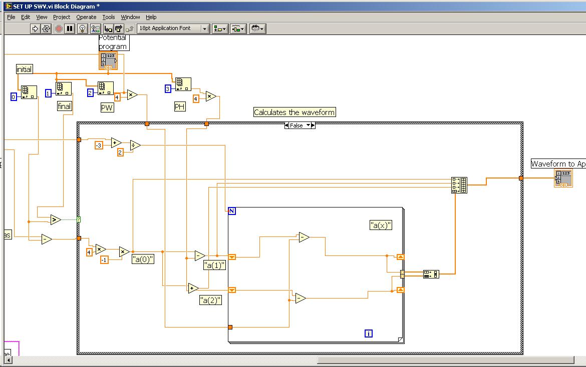
"Set Up SWV.vi"
This vi sends the commands which tell the potentiostat to enter arbitrary waveform mode, and which sets the source curve and processing curve to 0 (to accept the incoming waveform), and the destination curve to 3 (for current data collected). It sets the BIAS DAC on the potentiostat (i.e. a fixed starting point) to the average of the initial and final potential. It calculates the waveform which will be downloaded into the source curve (maximum 3050 points... I left a few points spare just in case). The source curve will be applied by the modulation DAC. The potentiostat has two DAC's, the sum of whose values determine the applied potential.
This vi also sets the sensitivity, turns any filtering off, and readies the potentiostat to take the scan.
Here is a screen shot of some of the "Send" commands

Here is a screen shot of the portion which calculates the waveform:
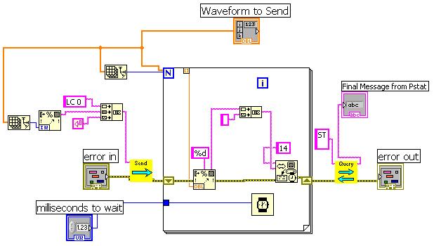
"EXPORT.VI"
The waveform calculated by "Set Up SWV.vi" is an array which is downloaded one point at a time into the Potentiostat's memory by "EXPORT.VI". The "LC" command is used to specify the location of the first point in memory (position zero) and the number of points for the potentiostat to expect. Each number in the array is converted from an integer to text and then sent to the potentiostat followed by a carriage return, so as not to overload the potentiostat's buffer. The transfer ends up being surprisingly fast, even with a millisecond delay time inserted between each point.
This vi also has the first instance in the suite of programs of "QUERY.vi". The "QUERY.vi" is used to send commands to the potentiostat which elicit a response. This instance sends the "ST" command to the potentiostat, which causes the potentiostat to report its error status and then reset its error status. You may notice that the "command error" light of the potentiostat flashes on briefly during "EXPORT.VI". This error seems to be due to an extra character being sent to the potentiostat after the download of bona fide waveform points is complete. The "ST" command returns a "command error", but then resets the error status so the potentiostat is fine. This error does not affect the potentiostat in any way except to make th eerror light to come on briefly. If it can be eliminated, an update will be posted.
Here is a screenshot of the entire back panel:
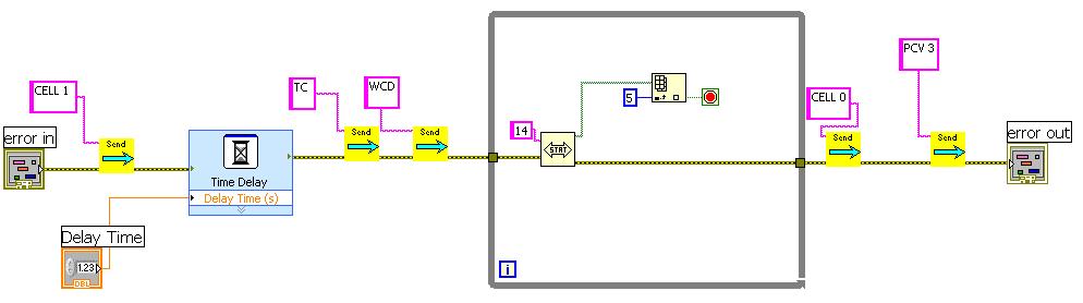
"RUN SWV.vi"
This vi (note the stylish icon!) turns the cell on, waits for the delay time, then starts data aquisition. A while loop causes the program to pauses during data aquisition. While status bit 5 (sweep done) is not set, the loop continues. In previous incarnations of this program, status bit 2 (curve done) was checked... the two are not the same, which resulted in an artificial delay being necessary. By checking status bit 5, there is no artificial delay, or annoying "dead time" at the end of the scan befor the transfer of current data to to PC happens.
Here is a screenshot of the back panel:
"EXTRACT.vi"
This vi uses the DC (download curve) command to tell the potentiostat to send data from the processing curve (curve 3) to the computer. Status bit 7 is checked to make sure the data is ready to be sent before the GPIB write command is used. The "talk" light is often on after this vi completes, which indicates that the potentiostat has something more to say, but its output buffer seems to be empty. "QUERY.vi" is used to request the status (ST) after "EXTRACT.vi" runs. This action usually resets the talk/listen status so the light goes off and the potentiostat is ready for the next scan.
If the talk light is on for too long, the potentistat will sometimes "hang" on the next scan... Cycle the power off and on again. This type of problem is much more rare now that there are fewer errors in the program.
After "EXTRACT.vi" is called, the "Square_Wave_Voltammetry.vi" processes the x and y axis data (X-axis: applied waveform is converted to mV and is added to bias potential, Y-axis: Current range info is used to convert the current readings into units of amps). This data is saved as a spreadsheet file, and the user is prompted for a filename. The filename is sent to "Display_SWV.vi" and then displayed on the main vi front panel, and the potentiostat is re-initialized.
"Display_SWV.vi" This vi can be used independently to view data previously collected!
Here is a screenshot of the front panel:

This vi reads in the data from the spreadsheet file. The spreadsheet file format is ASCII potential, current couples with even-numbered lines corresponding to forward data, and even-numbered lines corresponding to reverse data. The vi separates the data into three X,Y arrays, which are displayed on the graph. The couples are:
(1) Efor, Ifor
(2) Erev, Irev
(3) (Efor+Erev)/2 , (Ifor-Irev) (standard scan)
The difference in the peak potentials for the forward scan and the reverse scan should be twice the pulse height, rather than 59 mV as it is in CV.
For data recorded with low background current and small IR losses, the reversibility can be calculated as
reversibility = 1.5(Irev/Ifor) as described in the supporting material in Shaw et al, Organometallics, 23, 2205. This procedure worked out well when we used a 250 micron Pt disk electrode, although background current subtraction can be used to aleviate some of the problem.
If you see a flat line instead of a peak for the forward plot, then you should rerun the scan at a lower current sensitivity because the current went offscale. This advice is especially important even if the differential plot looks "OK" because it is (in reality) distorted. If both forward and reverse current are offscale, the differential plot will also appear clipped. Be careful at the solvent limits because if the forward peak is constant/offscale/maxed out, and the reverse current increases, an artifict that looks like a peak may show up in the differential scan. This problem has invalidated some results presented at Thesis defenses and has meant some (thankfully minor) re-writes for the individuals involved! Such problems can easily be detected if you look at all three plots, which is why the default view for this program shows them.
Each array is available at a terminal in the icon, so this vi can be incorporated into another vi which might save all three arrays as separate spreadsheet files. Such files can be easily imported into Excel to make publication-quality graphs.
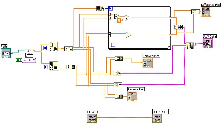
Here is a screenshot of the rear panel, which is very straightforward, although there are a bunch of crossing lines...
WHY Square Wave Voltammetry AT ALL!
My experience has been that SWV is a technique that provides information that is complementary to CV. The response to follow up reactions, especially to second-order follow up reactions, is quite different for the two techniques. The differences in the response can lead to more firm mechanistic conclusions.
SWV is also more sensitive than CV. The differential nature of the technique provides an even baseline so that peaks are easily discernable at concentrations that cause CV problems. For example, we can easily obtain useful data on 0.1 mM solutions of metalloporphyrins. Similar quality CV data required concentrations ten times greater. This sensitivity can be beneficial in mechanistic studies which use catalytic second-order reactions (electrocatalysis) to study reaction rates... At 0.1 mM concentrations, second order reactions with very large rate constants can be studied.
This program is an update of the "Sabrina.bas" Quickbasic program developed at the University of Vermont to run SWV, and it is "Sabrina-approved."
The data shown on the front panel is from a 3 mM solution of K4[Fe(CN)6] in 0.2 M KCl.
If you find these and the other program posted here useful, please reference where you got them in your Thesis, Dissertation, papers, etc.
Previous and current (CHE 0911537) support by NSF is gratefully acknowledged for this work.
**This document has been updated to meet the current required format for the NI Code Exchange.**
Example code from the Example Code Exchange in the NI Community is licensed with the MIT license.
