- Document History
- Subscribe to RSS Feed
- Mark as New
- Mark as Read
- Bookmark
- Subscribe
- Printer Friendly Page
- Report to a Moderator
- Subscribe to RSS Feed
- Mark as New
- Mark as Read
- Bookmark
- Subscribe
- Printer Friendly Page
- Report to a Moderator
PID Tutorial - LabVIEW for FRC
PID Tutorial
Contents
- Control Systems Review
- Introduction to PID
- Effective Use of PID in Robotics Systems
- Using PID in LabVIEW
- Tuning a Controller
- Conclusions
- Additional Resources
This article goes over a brief review of control systems and proceeds to cover PID theory, tuning basics and how to implement them using LabVIEW.
1. Control Systems Review
Control systems exist in everyday life, from robots to cars to even the human body. A control system aims to provide a desired response by changing its output based on its input. For instance, if you feel cold (input), your body will shiver to drive your body temperature back up (desired output).
A control system can be classified as either ‘open loop’ or ‘closed loop’:
An open loop control system, shown below in Figure 1, uses a controller to produce a signal that changes the overall output of the system. Note that here, there is no way for the controller to know what the system output (known as feedback) – the control action is independent of the desired output.

Figure 1. An open loop control system with no feedback.
A closed loop control system, shown in Figure 2, uses feedback to determine what the new output value should be. It takes the difference between the initial input (known as the reference) and the measured output and based on this difference (the error), performs the necessary steps to bring the output closer to what is desired. In most control applications (and ideally yours) a closed feedback loop will be used since it is more accurate (although generally more difficult to design and more expensive).
Figure 2. A closed loop control system uses feedback to drive the output to the desired value.
2. Introduction to PID
Proportional-Integral-Derivative (PID) control is used in a closed control feedback loop to regulate a process, such as the motion of a motor or the flow through a valve. It is the most common control algorithm used in industry and has been universally accepted in industrial control. The popularity of PID controllers can be attributed partly to their robust performance in a wide range of operating conditions and partly to their functional simplicity, which allows engineers to operate them in a simple, straightforward manner. Using PID control will make your robot design more stable, robust, and allows you to improve response characteristics.
As the name suggests, a PID algorithm consists of three basic coefficients: proportional, integral, and derivative, denoted below in Figure 3 as KP, KI, and Kd, respectively. These coefficients, called gains, alter the error signal fed back into the controller to determine the actuating signal. The gain values can be changed to achieve an optimal system response (a process called tuning, to be discussed in section 6).
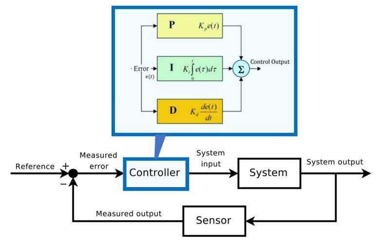
To implement a PID controller into the system, the sensor output is read (also called the process variable) with a sensor and compared to the reference value (also called the setpoint). The comparison of the reference and the measured output results in an error value which is used by the PID controller to calculate proportional, integral, and derivative responses. These three responses are then summed to obtain the output of the controller. The output of the PID controller is then used as an input to the system you wish to control, changing some aspect of the system. For example, if you are controlling a motor, the controller would provide more or less current. If you are controlling the flow of a fluid, the controller would cause a valve to open or close. The system output is then measured again and the whole process repeats. One completion of this process is called an iteration through the control loop.
A PID controller works by continuously measuring the output of your system and providing corrective input calculated from the PID control algorithm. The PID controller is scalable and tunable. It is scalable because you can implement a simpler controller by just using the proportional gain, or a combination of the proportional gain and either the integral or derivative gain (P, PI, PD, or PID controllers), where each configuration has its own advantages. The system is tunable because you can adjust the P, I, and D gains to tune the controller for your specific system application.
3. Effective Use of PID in Robotics Systems
PID algorithms are used in industry in a variety of control systems. In robotics and for FRC specifically, you will commonly see PID implemented for motion control, either for drive train motors or for other servo actuators. Before you decide to use PID control on your robot, you will want to consider a couple of different factors to evaluate if PID is warranted:
3a. Do you need PID in the first place?
- If your system doesn't exhibit error outside of your acceptable performance parameters...
- If all possible inputs to the system cannot result in undesired or possibly dangerous behavior…
- If you don't need to improve the response of your system...
…then you don't really need PID control, and your time is probably better spent on other areas of your robot.
3b. Is the system you are trying to control linear?
PID control is only effective for linear systems. If you have a system with non-linear response, the PID gains that are effective in tuning your system for one section of the response curve will not be valid for other parts of the response curve, resulting in erratic and uncontrolled behavior of your system. You will have to implement gain scheduling (applying different PID gains for each approximately linear section of the response curve) or PID in combination with feed-forward control to implement an effective control system.
Almost all motors will have documentation containing a Torque/Speed Curve. Use this curve to determine the linearity of your motor. A straight line with a constant slope indicates a linear motor. An exponential or polynomial curve indicates a non-linear motor. If you can't find information or specifications on your motor or other device, then you will need to perform a characterization of your system to determine its linearity.
3c. Do you have adequate real-world feedback?
You must have some method to measure the output of your system to provide feedback in calculating the system error. For motion systems this usually means an encoder or a gear tooth sensor.
Once you have determined that you have a linear system, and that you have some means of providing the necessary feedback, the next step is learning how to implement a PID controller.
4. Using PID in LabVIEW
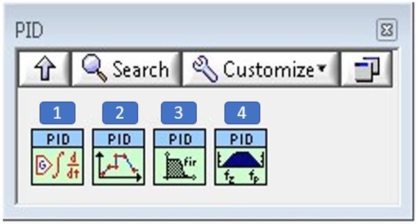
The LabVIEW FRC PID palette consists of four VIs:
- PID
- PID Setpoint Profile
- PID Control Input Filter
- PID Lead-Lag
Figure 4. The LabVIEW FRC PID palette.
The only VI you need to construct a regular PID controller is the PID VI. The other VIs in this palette implement more advanced functions and can be useful for some specific applications.
PID.vi
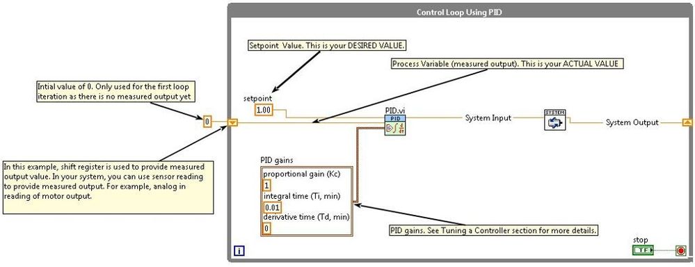
Implements a PID controller using a PID algorithm for simple PID applications that require an efficient algorithm. PID controller sample code is shown in Figure 5 below. This code demonstrates the use of PID.vi to implement a PID application. A shift register is used to store the system output value between iterations.
Figure 5. Implementation of the PID VI.
For sake of explanation, let’s pretend this code is used to control a motor that turns some wheel. Also, let’s pretend that we know that this motor will turn once per second if we apply 1A as its power source. Therefore, if you would like the motor to turn once per second your setpoint value for the PID.vi would be 1.
Wheel (motor) is exposed to different forces which will cause its turns to drop or increase. Despite that, we would like to maintain one turn per second. Therefore, we can use a sensor to measure turns of the wheel and use this data (measured output) as the process variable of PID.vi. PID VI will take the setpoint value, the process variable, and the PID gains to perform the PID algorithm. This process will yield an output which will be used as a system input (current applied to the motor) for the next cycle of the control loop. This process ensures that the motor is provided with a necessary current to turn once per second despite the force from outside sources.
PID Setpoint Profile.vi
You can use the Setpoint Profile VI to generate a setpoint profile. A setpoint profile is a premade set of data points that replaces your sensor input and can be useful when the system that you are controlling needs to go through a pre-defined series of states. Maybe you have a robotic arm that needs to complete a precise sequence of moves to pick up and place an object onto a raised platform. You can use setpoint profiling to define this sequence of movements, so that your robot’s behavior is repeatable and predictable; the arm will be in a specified position at a specified time. This method can be quicker and more precise than human control. It’s handy for autonomous tasks, as you can set up your program to trigger a certain profile based on input from other systems on your robot.
PID Setpoint Profile.vi Help Page
PID Control Input Filter.vi
The Input Filter VI implements a low-pass filter and can be used to filter out high-frequency noise from your process variable signal. Noise on the process variable line can result in undesirable fluctuations in the PID output.
PID Control Input Filter.vi Help Page
PID Lead-Lag.vi
The PID Lead-Lag VI uses a positional algorithm that approximates a true exponential lead/lag. Lead-Lag control is often used in feed-forward control schemes, as a dynamic compensator. This is in direct contrast to the PID algorithm, which is used in feedback systems. If you have a feed-forward controller, use the Lead-Lag VI in place of the PID VI.
5. Tuning a Controller
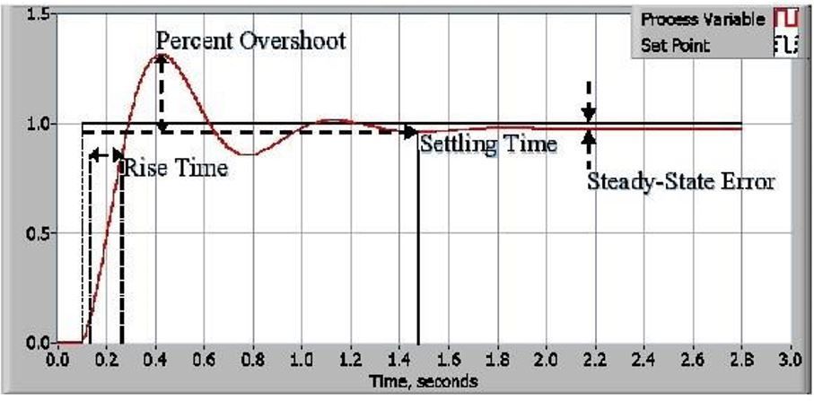
A PID controller needs to be tuned (PID gains set to appropriate values for your specific system) to function properly. The performance of your control system is defined by a set of measurements made when applying a specific input step function as the set point command variable (going from 0 to 100% of the output value instantaneously) and then measuring the response of the process variable. The key performance indicators for a PID-controlled system are the following:
Rise Time – How long it takes for the process variable to initially reach the desired set point value
Percent Overshoot – How much the process variable rises above the desired set point
Settling Time – How long it takes for the process variable to achieve ‘steady state’, where the error remains within a specific range of values (for instance, 5%)
Steady-State Error – How much the process variable differs from the set point once it has settled into steady state
These measurements are shown in the graph of a system’s response to a step input below in Figure 6.
Figure 6. The PID-controlled response of a system output compared with the set point.
Tuning your controller requires you to change the P, I, and D coefficient values to best achieve the response you want. Table 1 below shows the trade-offs of increasing each coefficient value. These correlations will not always hold true, since each coefficient may rely on one another, but they may be helpful when initially tuning your system.
Table 1. PID coefficient effects on performance parameters
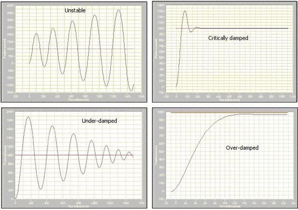
Additionally, you may desire an over-damped, critically damped, or under-damped system when tuning. In most robotics applications, overshoot is unacceptable and may cause damage to the system. Most robotics systems are over-damped so that they never overshoot their setpoint. The goal of tuning such systems is decreasing the rise-time and steady-state error to achieve the best possible performance. These types of responses are shown below in Figure 7.
Figure 7: System damping examples
- An unstable system produces an oscillatory, exponentially diverging step response. This kind of system never settles down; in fact, the oscillations tend to worsen over time.
- An under-damped system produces a slight oscillatory response that eventually dampens out. An under-damped system is characterized by a large overshoot, a long settling time, and short peak and rise times.
- A critically damped system response provides a balanced medium between over- and under-damping. This type of system response balances response time and damping effects. A critically damped system is characterized by low overshoot, shorter rise and settling times when compared to over-damped systems and longer peak times when compared to under-damped systems.
- An over-damped system produces a smoother, slower step response. An over-damped system is characterized by no overshoot and long rise and settling times.
Tuning your system requires changing the gains and testing them out, noting the key parameters previously mentioned. One method to tune a system would be to keep increasing the Proportional gain, until the system response reaches the value of the setpoint and then adjust the Integral and/or Derivative gains to achieve a better-fitting response.
6. Conclusion
Congratulations, you now have a basic working knowledge of PID theory as it relates to FRC and robotic systems. Leverage the power of LabVIEW and use PID control to build a better robot!
To learn more about PID control theory, as well as some advanced topics like gain scheduling and lead-lag controllers, check out the additional resources below, along with the LabVIEW shipping examples (LabVIEW Help menu»Find Examples). If you have suggestions on how to improve this tutorial, please add them to the comments section below so that we can continue to improve our documentation and training resources.
7. Additional Resources
“Control Systems-Introduction”: Basic overview of control systems and comparisons between closed and open loop systems.
https://www.tutorialspoint.com/control_systems/control_systems_introduction.htm
“PID Theory Explained”: Provides a very thorough explanation of control systems, PID theory/tuning/considerations, and LabVIEW implementation.
PID controller: Dives deep into the history and math of PID.

